General relativity
In general relativity gravity is described by a four dimensional space-time endowed with a Lorentzian (non-flat) metric. The four dimensional space-time can have a non-trivial curvature and mayhap even a non-trivial topology and it hence become necessary to discuss manifolds.Manifolds
Since (differentiable) manifolds is a central concept in general relativity, see e.g. \cite{wal-84}, \cite{sch-80} (as in all field theories, see e.g. \cite{Lan-lif-80}), they need to be properly defined, however, one can start with an intuitive description: A manifold is a set made up of pieces (or charts) that ``look like" open subsets of $\mathbb{R}^n$ that can be "sewn together" smoothly. Thus although locally the manifold looks like $\mathbb{R}^n$, on a global scale it may have a non-trivial topology. A simple example is the surface of a 2-sphere, $\mathbb{S}^2$; incidentally, note that a 2-sphere can not be covered by a single chart in $\mathbb{R}^2$ in a continuous one-to-one manner, but several charts can, and then these charts can be "sewn together" smoothly creating an atlas. Thus, since the surface of the Earth is roughly a sphere, and hence has $\mathbb{S}^2$ topology, one cannot have a global map on a single piece of paper, one is forced to use several pieces of paper that describe overlapping local regions in order to cover the whole surface completely. More formally a manifold is defined asAn n-dimensional, $C^\infty$, real manifold $M$ is a set together with a collection of subsets $\{ O_\alpha \}$ satisfying the following properties:The manifolds being used in general relativity are four-dimensional Riemannian manifolds, or rather pseudo-Riemannian manifolds, which is a generalization of Riemannian manifolds, since distances need not be positive definite.
- Each $p \in M$ lies in at least one $O_\alpha$, i.e. the $\{ O_\alpha \}$ covers $M$.
- For each $\alpha$ there is a one-to-one, onto, map $\psi _\alpha : O_\alpha \rightarrow U_\alpha$, where $U_\alpha$ is an open subset of $\mathbb{R}^n$.
- If any two sets $O_\alpha$ and $O_\beta$ overlap, $O_\alpha \cap O_\beta \neq \varnothing$, we can consider the map $\psi_\beta \circ \psi_\alpha ^{-1}$ which takes points in $\psi_\alpha [O_\alpha \cap O_\beta] \subset U_\alpha \subset \mathbb{R}^n$ to points $\psi_\beta [O_\alpha \cap O_\beta] \subset U_\beta \subset \mathbb{R}^n$. We require these subsets of $\mathbb{R}^n$ to be open and this map to be $C^\infty$.
Tangent spaces
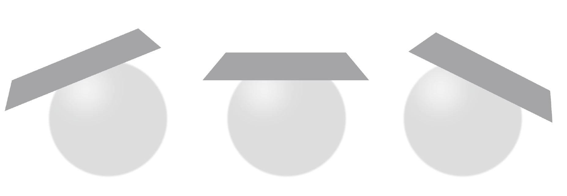
Any point of a manifold has a tangent space associated with it \cite{sch-80}. One can easily visualize the tangent plane at a point that a 2-sphere imbedded in $\mathbb{R}^3$ has, see Figure
Tensors
In general relativity tensors play a crucial r\^{o}le since they are mathematical objects used for describing nature without any preferred coordinate systems. To define tensors one needs to begin by defining scalars, i.e. numbers, vectors, and so-called dual vectors, see e.g. \cite{sch-80}, \cite{fos-nig-79} and \cite{car-03}.Scalars
A scalar $\phi \in \mathbb{R}$, is any real number.Vectors
Considering a coordinate chart $x^\mu$, there exists an obvious independent set of $n$-directional derivatives at a point $P$, the partial derivatives $\partial _\mu$, and thus the partial derivative operators $\left \{ \partial _\mu \right \}$ at $P$ form a basis for the tangent space $T_P(M)$. To prove this one has to show that any directional derivative can be decomposed into real numbers and partial derivatives, this is rather easily done by showing that for an arbitrary (scalar-)function $f$ one has that \[ \frac{d}{d\lambda} f = \frac{dx^\mu}{d\lambda}\partial_\mu f \] which implies that \[ \frac{d}{d\lambda} = \frac{dx^\mu}{d\lambda}\partial_\mu, \] since $f$ is arbitrary; to avoid cluttered notation the index $P$ has been dropped. Thus one can describe $T_P(M)$ in a given basis $\left \{ e_\mu \right \} = \left \{ \partial_\mu \right \}$, which is known as a coordinate basis, since one has basis vectors pointing along the coordinate axes. One reason for using a coordinate basis is that transformations under a change of coordinates is rather straight forward, changing from $x^\mu$ to $x^{\mu '}$ yields the transformation \[ \partial_{\mu '} = X^\mu {}_{\mu '}\partial _\mu, \] where \[ X^\mu {}_{\mu '} = \frac{\partial x^\mu}{\partial x^{\mu '}}. \] Using a coordinate basis one can describe an arbitrary vector $\vec V$ by its components $V^\mu$ as \[ \vec V = V^\mu \partial _\mu. \] Requiring that $\vec V$ is unchanged under a change of coordinates yields \[ \begin{aligned} \vec V = V^\mu \partial_\mu =& V^{\mu '} \partial_{\mu '}\\ =& V^{\mu '} X^\mu {}_{\mu '} \partial _\mu, \end{aligned} \] and thus $V^\mu = X^\mu{}_{\mu '} V^{\mu '}$. Since $X^{\mu '}{}_\mu = \frac{\partial x^{\mu '}}{\partial x ^\mu}$ is the inverse of $X^\mu{}_{\mu '} = \frac{\partial x^\mu}{\partial x ^{\mu '}}$ it follows that \[ V^{\mu '} = X^{\mu '}{}_{\mu} V^\mu. \] Vector spaces like $T_P$ are linear; one can add vectors and multiply them with scalars: \[ (\phi + \varphi)( V^\mu + W^\mu ) = \phi V^\mu + \varphi V^\mu + \phi W^\mu + \varphi W^\mu \] where, $\phi ,\varphi \in \mathbb{R}$ and $V^\mu ,W^\mu \in T_P$.Dual vectors
The best way to think of dual vectors is in terms of a tangent space $T^*_P$, which give linear maps $\omega: T_P \rightarrow \mathbb{R}$, s.t. \[ \omega_\mu(\phi V^\mu + \varphi W^\mu) = \phi \omega_\mu(V^\mu) + \varphi \omega_\mu(W^\mu) \in \mathbb{R} \] and \[ (\phi \omega_\mu + \varphi \varpi_\mu)(V^\mu) = \phi \omega_\mu(V^\mu) + \varphi \varpi_\mu(V^\mu) \in \mathbb{R} \] where $\phi, \varphi \in \mathbb{R}$, $V^\mu, W^\mu \in T_P$ and $\omega, \varpi \in T^*_P$ The gradient of $f$, with notation $df$, is a dual vector since the gradient $df$ acting on a vector $d/d\lambda$ is defined to yield \begin{equation}\label{directional} df \left ( \frac{d}{d\lambda} \right ) = \frac{df}{d\lambda}, \end{equation} which is the same as the directional derivative. In the same way that partial derivatives form a basis for $T_P$, the gradient along the coordinate functions $x^\mu$ forms a basis for $T^*_P$, and one can use (\ref{directional}) to find that \[ dx^\mu \partial _\nu = \frac{\partial x^\mu}{\partial x^\nu} = \delta ^\mu{}_\nu, \] where $\delta ^\mu{}_\nu$ is the Kronecker delta described by \[ \delta ^\mu {}_\nu = \left\{\begin{matrix} 1, & \mbox{if } \mu = \nu \\ 0, & \mbox{if } \mu \ne \nu \end{matrix} \quad. \right. \] Hence the set of gradients $\left \{ dx^\mu \right \}$ is an appropriate basis, and one can expand dual vectors into components as $\vec \omega = \omega _\mu dx^\mu$. Under a coordinate transformation the dual vectors transforms as \[ dx^{\mu '} = \frac{\partial x^{\mu '}}{\partial x^\mu} dx^\mu= X^{\mu '}{}_\mu dx^\mu, \] and hence components transform as \[ \omega_{\mu '} = X^\mu{}_{\mu '}\omega _\mu. \]Tensors
A rank $(r,s)$ tensor $\vec T$ with components $T^{\mu_1 \cdots \mu_r}{}_{\nu_1 \cdots \nu_s}$, is a tensor with $r$ ``slots" in which one can insert dual vectors and $s$ ``slots" where one can insert vectors to create a scalar. \[ \vec T = T^{\mu_1 \cdots \mu_r}{}_{\nu_1 \cdots \nu_r} \underbrace{\partial_{\mu_1} \otimes \cdots \otimes \partial_{\mu_r}}_{r \textrm{ slots for dual vectors }} \otimes \underbrace{dx^{\nu_1} \otimes \cdots \otimes dx^{\nu_s}}_{s \textrm{ slots for vectors}}. \] Tensors extend the classical notions of scalars, vectors/dual vectors; in the same way a dual vector is a linear map from vectors to $\mathbb{R}$, a tensor of rank $(r,s)$ is a multilinear map from a collection of vectors and dual vectors to $\mathbb{R}$. Multilinear means that it is linear in all its arguments; i.e. a tensor of rank $(1,1)$ satisfies- $\vec T(a \vec V,\vec \omega) = a \vec T (\vec V, \vec \omega)$,\, $\vec T(\vec V, c \vec \omega) = c \vec T (\vec V, \vec \omega)$
- $\vec T(\vec V + \vec W, \vec \omega) = \vec T (\vec V, \vec \omega) + \vec T(\vec W, \vec \omega)$, $\vec T(\vec V, \vec \omega + \vec \varphi) = \vec T (\vec V, \vec \omega) + \vec T(\vec V, \vec \varphi)$
Tensor algebra
Tensor products/outer products
If one has a tensor with rank $(r,0)$ $A^{\mu_1 \cdots \mu_r}$, and a tensor with rank $(0,s)$ $B_{\nu_1 \cdots \nu_s}$, one can introduce the so-called tensor product or outer product, \[ A^{\mu_1 \cdots \mu_r} B_{\nu_1 \cdots \nu_s} = C^{\mu_1 \cdots \mu_r}{} _{\nu_1 \cdots \nu_s}, \] to obtain a new tensor $C^{\mu_1 \cdots \mu_r}{}_{\nu_1 \cdots \nu_s}$ of rank $(r,s)$.Contractions/inner products
Consider a tensor of rank $(r+1,s+1)$ $V^{\mu_1 \cdots \mu_r \nu}{} _{\sigma \rho_1 \cdots \rho_s}$; by summing over $\nu$ and $\sigma$ one obtains $V^{\mu_1 \cdots \mu_r \nu}{}_{\nu \rho_1 \cdots \rho_s}$, which transforms as a tensor of rank $(r,s)$ and thus yields a tensor which we denote by $V^{\mu_1 \cdots \mu_r}{} _{\rho_1 \cdots \rho_s}$, i.e. \[ V^{\mu_1 \cdots \mu_r }{} _{\rho_1 \cdots \rho_s} = V^{\mu_1 \cdots \mu_r \nu}{}_{\nu \rho_1 \cdots \rho_s}. \]Symmetry relations
A rank $(2,0)$ tensor is symmetric if \[ T^{\mu \nu} = T^{\nu \mu} \] and a rank $(2,0)$ tensor is antisymmetric if \[ T^{\mu \nu} = -T^{\nu \mu} \] One sometimes wants, for various reasons, to decompose tensors into symmetric or anti-symmetric parts; this can be accomplished as follows. Starting with symmetrization of a general tensor, one needs to take the average over all its transposes, \[ V_{\left (\mu_1 \ldots \mu_n \right )} = \frac{1}{n!}\sum_\pi V_{\mu_{\pi(1)} \ldots \mu_{\pi(n)}} \] where the sum is taken over all possible permutations $\pi$, e.g. the symmetric part of a second rank $V_{\mu \nu}$ tensor thus becomes \[ V_{(\mu \nu)} = \frac{1}{2} \left ( V_{\mu \nu} + V_{\nu \mu} \right ), \] while a third rank tensor yields \[ V_{(\mu \nu \lambda)} = \frac{1}{6} \left ( V_{\mu \nu \lambda} + V_{\nu \lambda \mu} + V_{\lambda \mu \nu } + V_{\nu \mu \lambda} + V_{\mu \lambda \nu} + V_{\lambda \nu \mu} \right ). \] This is also applicable to composite tensors, e.g., \[ A^{(\mu} B^{\nu)} = \frac{1}{2} \left ( A^\mu B^\nu + A^\nu B^\mu \right ). \] In a similar way one accomplish anti-symmetrization of a tensor, $V_{\mu_1 \cdots \mu_n}$: \[ V_{\left [\mu_1 \ldots \mu_n \right]} = \frac{1}{n!}\sum_\pi \delta_\pi V_{\mu_{\pi(1)} \ldots \mu_{\pi(n)}} \] where \[ \delta_\pi = \left \{ \begin{array}{l} +1 \ \textrm{ for even permutations}\\ -1 \ \textrm{ for odd permutations}\\ \end{array} \right. . \] Thus anti-symmetrization of a second rank tensor $V_{\mu \nu}$ is given by \[ V_{[\mu \nu]} = \frac{1}{2} \left ( V_{\mu \nu} - V_{\nu \mu} \right ), \] while anti-symmetrization of a third rank tensor $V_{\mu \nu \lambda}$ yields \[ V_{[\mu \nu \lambda]} = \frac{1}{6} \left ( V_{\mu \nu \lambda} + V_{\nu \lambda \mu} + V_{\lambda \mu \nu } - V_{\nu \mu \lambda} - V_{\mu \lambda \nu} - V_{\lambda \nu \mu} \right ). \] It is also possible to symmetrize some parts of a tensor, and anti-symmetrize another part \[ V^{\left (\mu_1 \ldots \mu_n \right )}{}_{\left [\nu_1 \ldots \nu_n \right]} = \frac{1}{n!}\sum_{\pi, \gamma} \delta_\pi V^{\mu_{\gamma (1)} \ldots \mu_{\gamma (n)}}{}_{\quad \nu_{\pi(1)} \ldots \nu_{\pi(n)}} \] which in the $\left ( 2, 2 \right )$ case leads to \[ V^{\left (\mu \nu \right )}{}_{\left [\alpha \beta \right]} = \frac{1}{4}\left ( V^{\mu \nu}{}_{\alpha \beta} + V^{\nu \mu}{}_{\alpha \beta} - V^{\mu \nu}{}_{\beta \alpha} - V^{\nu \mu}{}_{\beta \alpha}\right ). \] Here are some short examples of tensor symmetry relations:- $V_{\mu \nu} = V_{(\mu \nu)} + V_{[\mu \nu]}$.
- $A_{(\mu \nu)} = 0$, gives that $A_{\mu \nu}$ is an anti symmetric-tensor.
- $S_{[\mu \nu]} = 0$, gives that $S_{\mu \nu}$ is an symmetric tensor.
- $A^{\mu \nu} S_{\mu \nu} = 0 \quad \forall \quad A^{\mu \nu}, S_{\mu \nu}$, s.t. $A^{\mu \nu} = A^{[\mu \nu]}$ and $S_{\mu \nu} = S_{(\mu \nu)}$.
Tensor fields
In general relativity one is primarily interested in tensor fields. To describe what a tensor field is one starts by using the dual space $T_P ^*(M)$ defined in \ref{dual-vectors}, which makes it possible to build spaces of the form $\left( T^m{}_{n} \right ) _P (M)$. Then a tensor field is defined by defining a tensor at each point $P$ on the manifold $M$; the set of all tensor fields on $M$ is denoted $T^m {}_{n} (M)$, for a more exhaustive explanation of this description, see \cite{sch-80}. Alternatively to being defined as multilinear maps at each point $P$ on $M$, a tensor field can defined by its transformation properties, see e.g. \cite{car-03}, \cite{fos-nig-79}. In a coordinate neighborhood the components of a tensor field may be regarded as a function of the coordinates, and is by definition transformed according to \begin{equation}\label{transform} T^{\mu ' \cdots \nu '}{}_{\alpha ' \cdots \beta '} = X^{\mu '}_{~\mu} \cdots X^{\nu '}_{~\nu} X^{\alpha}_{~\alpha '} \cdots X^{\beta}_{~\beta '} T^{\mu \cdots \nu}{}_{\alpha \cdots \beta}. \end{equation}Differentiation
Differentiation is usually an important concept, but on an arbitrary manifold there are differences from how it is done in flat space, which, perhaps, is the familiar setting for the undergraduate student. Starting with a scalar $\phi$, the chain rule gives \[ \partial _{\mu '} \phi = X^\mu{}_{\mu '} \partial _\mu \phi, \] and hence $\partial _{\mu '} \phi$ transforms as a vector according to (\ref{transform}). Now applying the chain rule to a vector with components $V^{\nu}$ gives \begin{equation}\label{differentiation-vector} \begin{aligned} \partial _{\mu '} V^{\nu '} &= X^\mu{}_{\mu '} \partial _\mu \left ( X^{\nu '}{}_{\nu} V^\nu \right )\\ &= X^\mu{}_{\mu '} X^{\nu '}{}_{\nu} \left( {\partial _\mu V^\nu} \right) + X^{\mu}{}_{\mu '} \left ( \partial _\mu X^{\nu '}{}_{\nu} \right )V^\nu\\ &=\frac{\partial x^{\mu}}{\partial x^{\mu '}} \frac{\partial x^{\nu '}}{\partial x^{\nu}} \left ( \partial _\mu V^\nu \right ) + \frac{\partial x^\mu}{\partial x^{\mu '}} \frac{\partial ^2 x^{\nu '}}{\partial x^{\mu} \partial x^{\nu}} V^\nu \end{aligned} \end{equation} and hence $\partial _{\mu '} V^{\nu '}$ does not transform accordingly to (\ref{transform}), and is thus not a tensor. Therefore one needs to invent a new object \cite{Wei-72}, the first thing to do is defining an object $\Gamma ^\lambda {}_{\mu \nu}$ that transforms as \begin{equation}\label{transformation-Gamma} \Gamma ^{\lambda '}{}_{\mu ' \nu '} = \frac{\partial x^{\lambda '}}{\partial x^{\lambda}} \frac{\partial x^{\mu}}{\partial x^{\mu '}} \frac{\partial x^{\nu}}{\partial x^{\nu '}} \Gamma ^{\lambda}{}_{\mu \nu} - \frac{\partial x^{\nu}}{\partial x^{\nu '}} \frac{\partial x^{\mu}}{\partial x^{\mu '}} \frac{\partial ^2 x^{\lambda '}}{\partial x^{\lambda} \partial x^{\nu}}. \end{equation} Now applying (\ref{transformation-Gamma}) to a vector $V^\nu$ yields \begin{equation}\label{Gamma-vector} \begin{aligned} \Gamma ^{\lambda '}{}_{\mu ' \nu '} V^{\nu '} =& \left ( \frac{\partial x^{\lambda '}}{\partial x^{\lambda}} \frac{\partial x^{\mu}}{\partial x^{\mu '}} \frac{\partial x^{\nu}}{\partial x^{\nu '}} \Gamma ^{\lambda}{}_{\mu \nu} - \frac{\partial x^{\nu}}{\partial x^{\nu '}} \frac{\partial x^{\mu}}{\partial x^{\mu '}} \frac{\partial ^2 x^{\lambda '}}{\partial x^{\lambda} \partial x^{\nu}} \right ) \frac{\partial x^{\nu '}}{\partial x^\sigma} V^\sigma\\ =& \frac{\partial x^{\lambda '}}{\partial x^{\lambda}} \frac{\partial x^{\mu}}{\partial x^{\mu '}} \Gamma ^{\lambda}{}_{\mu \nu} V^\nu - \frac{\partial ^2 x^{\lambda '}}{\partial x^{\lambda} \partial x^{\nu}} \frac{\partial x^{\mu}}{\partial x^{\mu '}} V^\nu. \end{aligned} \end{equation} By adding (\ref{differentiation-vector}) and (\ref{Gamma-vector}), one finds that the combination \[ \partial _{\mu '} V^{\lambda '} + \Gamma ^{\lambda '}{}_{\mu ' \nu '} V^{\nu '} = \frac{\partial x^{\lambda '}}{\partial x^{\lambda}} \frac{\partial x^{\mu}}{\partial x^{\mu '}} \left ( \partial _\mu V^\nu + \Gamma^{\lambda}{}_{\mu \nu} V^\nu \right ), \] transforms as a tensor according to (\ref{transform}). This motivates introducing the notation \begin{equation}\label{co-der1} \nabla_\mu V^\nu \equiv \partial _\mu V^\nu + \Gamma ^{\nu}{}_{\mu \kappa} V^\kappa, \end{equation} where $\nabla _\mu V^\nu$ is a tensor of rank $(1,1)$, and where $\nabla _\mu$ is known as a covariant derivative while $\Gamma ^{\lambda}{}_{\mu \nu}$ is known as an affine connection. By definition $\nabla _\mu f = \partial _\mu f$ for an arbitrary function, it follows that if one instead has a dual vector $V_\nu$, one can show that \begin{equation}\label{co-der2} \nabla _\mu V_\nu = \partial _\mu V_\nu - \Gamma _{~\mu \nu }^\lambda V_\lambda. \end{equation}Metric structures
The metric tensor
In general relativity gravity is described in terms of curved geometry. This means that one has to generalize the line element $ds^2 = \eta _{\mu \nu} dx^\mu dx^\nu$ to $ds^2 = g _{\mu \nu} dx^\mu dx^\nu$ where $g_{\mu \nu}$ depends on the manifold position. The metric $g_{\mu \nu}$; is a covariant tensor with rank $(0,2)$ that is symmetric and invertible. The inverse $g^{\mu \nu}$ by definition has the property \[ g^{\sigma \mu} g_{\mu \rho} = \delta ^\sigma {}_\rho. \] The metric tensor $g_{\mu \nu}$, and its inverse, provide isomorphisms between vector space and its dual, thus making it possible to raise and lower indices \[ V^\mu = g^{\mu \nu} V_\nu \quad V_\mu = g_{\mu \nu} V^\nu. \]The Christoffel symbol
In general relativity the covariant derivative of the metric (and its inverse) is required to be identically zero \begin{equation}\label{metric-compatability} \nabla _\sigma g_{\mu \nu } = \nabla _\sigma g^{\mu \nu } = 0. \end{equation} The components $\Gamma^{\lambda}{}_{\mu \nu}$ in (\ref{co-der1}) and (\ref{co-der2}) are called connection coefficients, but in general relativity one is interested in a special type of connection $\Gamma^{\lambda}{}_{\mu \nu}$, namely those that follow from the condition $(\ref{metric-compatability})$, which implies that \begin{equation}\label{Christoffel-1} \nabla _\rho g_{\mu \nu } = \partial _\rho g_{\mu \nu } - \Gamma _{\ \rho \mu }^\lambda g_{\lambda \nu } - \Gamma _{\ \rho \nu }^\lambda g_{\mu \lambda } =0, \end{equation} \begin{equation}\label{Christoffel-2} \nabla _\mu g_{\nu \rho } = \partial _\mu g_{\nu \rho } - \Gamma _{\ \mu \nu }^\lambda g_{\lambda \rho } - \Gamma _{\ \mu \rho }^\lambda g_{\nu \lambda } =0, \end{equation} \begin{equation}\label{Christoffel-3} \nabla _\nu g_{\rho \mu } = \partial _\nu g_{\rho \mu } - \Gamma _{\ \nu \rho }^\lambda g_{\lambda \mu } - \Gamma _{\ \nu \mu }^\lambda g_{\rho \lambda } =0; \end{equation} if one from (\ref{Christoffel-1}) subtracts (\ref{Christoffel-2}) \& (\ref{Christoffel-3}), and if one assumes a symmetric connection, i.e. $\Gamma ^\lambda _{\mu \nu} = 0$, \[ \partial _\rho g_{\mu \nu } - \partial _\mu g_{\nu \rho } - \partial _\nu g_{\rho \mu } + 2\Gamma _{\ \mu \nu }^\lambda g_{\rho \lambda } = 0, \] which can be rewritten as \begin{equation}\label{Christoffel} \Gamma ^\sigma _{\ \mu \nu } = \frac{1}{2}g^{\sigma \rho } \left( {\partial _\mu g_{\nu \rho } + \partial _\nu g_{\rho \mu } - \partial _\rho g_{\mu \nu } } \right). \end{equation} This particular form of $\Gamma^{\lambda}{}_{\mu \nu}$ is known as the Christoffel symbol.Parallel transport
Parallel transport is a rule for how vectors are transported along smooth curves in a manifold. In flat Euclidean space there is an ``obvious" simple rule: transport a vector and keep its Cartesian components constant. The problems arise when trying to parallel transport on a manifold, \cite{car-03}. The ``obviousness" in the Euclidean case is due to that Euclidean space is endowed with a lot of structure. We do not need all this structure in the general case, but we do need some, we need the affine connection $\Gamma^{\lambda}{}_{\mu \nu}$ which can be interpreted as a rule for how one parallel transport vectors. Start by considering an arbitrary curve $x^\mu(\lambda)$ with its tangent vector defined by $U^\mu = \frac{dx^\mu}{d\lambda}$. Then take an arbitrary vector $\vec V$ at a point $P$ on $x^\mu$, the connection then gives a rule of how to define $V^\mu$ along $x^\mu(\lambda)$, i.e. to parallel transport it \[ \nabla _{\vec U} V^\mu = U^\mu \nabla_\mu V^\mu + \Gamma^\mu _{~\alpha \beta} U^\alpha V^\beta = 0 \] where $\nabla _{\vec U}$ is the covariant derivative in the $\vec U$-direction.Geodesics
Geodesics are generalizations of straight lines to a case with non-Euclidean geometry. In terms of the covariant derivative geodesics are defined s.t. the tangent vectors along the geodesic curve remain parallel when transported along it, which formally is expressed as \[ \nabla _{\vec U} U^\mu = 0. \] If we use local coordinates, the geodesic equation take the form \begin{equation}\label{geodesic-eqn} \frac{d^2x^\lambda }{dt^2} + \Gamma^{\lambda}_{~\mu \nu }\frac{dx^\mu }{dt}\frac{dx^\nu }{dt} = 0. \end{equation} In general relativity test particles\footnote{Particles that are only affected by gravity, without producing any gravity or force fields.} follow geodesics; i.e. test particles allow us to probe space-time geometry and thus gravity.The Riemann curvature tensor
When watching a cylinder it looks round, and one could easily believe that it is a surface with curvature where e.g. Pythagoras theorem would not apply, but cutting it and rolling it out on the table without stretching or distorting it yields a flat surface, revealing that a cylinder is intrinsically flat, although it has extrinsic curvature when imbedded in 3-dimensional Euclidean space. However, it is impossible to roll out a sphere, a sphere is intrinsically curved, and hence e.g. triangles formed from geodesics have angular sums larger than $180^\circ$. In general relativity it is only the intrinsic geometry that interests us, how our four dimension looks in ten or eleven dimensions is completely irrelevant. Intrinsic curvature can be linked to the metric via the Christoffel symbol from (\ref{Christoffel}). The Riemann tensor is defined by \[ R^\sigma _{\ \mu \alpha \beta} \equiv \partial _\alpha \Gamma ^\sigma _{\ \mu \beta} - \partial _\beta \Gamma ^\sigma _{\ \mu \alpha} + \Gamma ^\sigma _{\ \alpha \lambda} \Gamma ^\lambda _{\ \mu \beta} - \Gamma ^\sigma _{\ \beta \lambda} \Gamma ^\lambda _{\ \mu \alpha}, \] where $\Gamma$ is the Christoffel symbol given by (\ref{Christoffel}). The Riemann tensor has $4^4 = 256$ components, but due to symmetries the number of independent components are actually $20$. The symmetries are most easily seen if one lowers the upper indices, i.e. \[ R_{\mu \nu \rho \sigma} = g_{\mu \lambda} R^\lambda _{\ \nu \rho \sigma}. \] It can be shown that the following symmetry relations hold: \[ \begin{aligned} R_{\mu \nu \rho \sigma } = R_{\left[ {\mu \nu } \right]\left[ {\rho \sigma } \right]} &= R_{\left[ {\rho \sigma } \right]\left[ {\mu \nu } \right]}, \\ R_{\mu \left[ {\nu \rho \sigma } \right]} &= 0. \\ \end{aligned} \] Thus, $R_{\mu \nu \rho \sigma}$ is anti-symmetric in $\mu , \nu$ and $\rho , \sigma$, and symmetric in exchange of $(\mu , \nu)$ for $(\rho , \sigma)$ and furthermore satisfies the so-called cyclic identity $R_{\mu \left [\nu \rho \sigma \right ]}$ which leads to that \[ R_{\left [ \mu \nu \rho \sigma \right ]} = 0. \]The Bianchi identities
There are two identities credited to Bianchi, the first is the already stated cyclic identity \[ R_{\mu \left[ {\nu \rho \sigma } \right]} = 0, \] also known as the algebraic Bianchi identity. The other Bianchi identity, also known as differential Bianchi identity, is \[ \nabla _{[\lambda } R_{\mu \nu ]\rho \sigma } = 0. \] The Riemann tensor contains all the information about the intrinsic curvature of the space time, but there are several contractions of it.The Ricci tensor
The Ricci tensor is a contraction of the Riemann tensor, and is, thanks to the Bianchi identities, symmetric \[ R_{\mu \nu} = R_{\nu \mu} = R^\lambda _{\ \mu \lambda \nu}. \]The Ricci scalar
The Ricci scalar is a contraction of the Ricci tensor, defined as follows \[ R = R^\mu{}_\mu = g^{\mu \nu}R_{\mu \nu}. \]The Einstein tensor
If the Bianchi identities are applied to the Ricci tensor one gets \[ \nabla _\lambda R_{\beta \nu} - \nabla _\nu R_{\beta \lambda} + \nabla _\mu R^\mu{}_{\beta \nu \lambda} = 0. \] Then contracting this with $g^{\beta \nu}$, and using the symmetry relations, one obtain \[ \nabla _\lambda R - \nabla _\mu R^\mu {}_\lambda - \nabla _\mu R^\mu{}_\lambda = 0, \] which can be written as \[ \nabla _\mu \left ( 2 R^\mu _{\ \lambda} - \delta ^\mu{}_\lambda R \right ) = 0. \] This motivates defining the so-called Einstein tensor $G_{\mu \nu}$, \[ G_{\mu \nu} \equiv R_{\mu \nu} - \frac{1}{2} g_{\mu \nu} R, \] which thus is symmetric, and satisfies \begin{equation}\label{G-conservation} \nabla _\mu G^\mu{}_\nu = 0. \end{equation}Einstein's field equations
"Matter tells space how to curve, and space tells matter how to move."Einstein's field equations are given by \[ G_{\mu \nu} = R_{\mu \nu} +\frac{1}{2}g_{\mu \nu}R = \kappa T_{\mu \nu}. \] and describe gravitation as a curvature of space-time caused by matter and energy; that is they determine the metric of space-time. On the left hand side of the field equations one has the Einstein tensor $G_{\mu \nu}$, and on the right hand side the so-called stress-energy tensor $T_{\mu \nu}$, the matter and energy content that acts as a source for gravity; $\kappa$ is a constant determined by the Newtonian limit of Einstein's field equations which yields $\kappa = 8 \pi$ (the Newtonian constant of gravitation, $G$, is set to 1), see e.g., \cite{car-03}, \cite{Wei-72}. The components of $T_{\mu \nu}$ can be physically interpreted as follows:-John Archibald Wheeler
- $T_{00}$ is the mass-energy density $\rho$, which includes mass and internal and kinetic energies.
- $T_{0i}$ is the energy flux.
- $T_{i0}$ is the momentum density.
- $T_{ii}$ (no sum) is the pressure, $p$.
- $T_{12}, T_{13}$, and $T_{23}$ describe shear stresses.
- $T_{21}, T_{31}$, and $T_{32}$ constitute the momentum flux.
- Vacuum: $T_{\mu \nu} = 0$.
- A perfect fluid: $T_{\mu \nu } = \left( {\rho + p} \right)u_\mu u_\nu + pg_{\mu \nu }$.
- An electromagnetic field: $T_{\mu \nu} = F_{\mu \alpha} g^{\alpha \beta} F_{\nu \beta} - \frac{1}{4} g_{\mu \nu} F_{\delta \gamma} F^{\delta \gamma}$.